Long-coherence biodynamic imaging using a common path system

Biodynamic imaging is a dynamic-contrast en-face holographic imaging technique²⁰ with high sensitivity to slow motions. Conventional microscopy techniques can only detect dynamics of features larger than its resolution limit, and in many microscopy techniques there are tradeoffs between the spatial and temporal resolution. Therefore, most microscopy techniques, including various forms of fluorescence microscopy, are unsuitable for observing microscopic movement on the scale of intracellular components, as either the spatial resolution or the temporal resolution is too coarse to detect such movement. Various forms of dynamic OCT methods use intensity fluctuations as a contrast medium, similar to biodynamic imaging of all forms, but the drawback of most dynamic OCT methods is that the image acquisition happens in the form of rasterized scans. The measurement of two adjacent pixels are offset in time, and the uncertainty in the timing of each measurement is different for each pixel. In contrast, the holography technique used in all forms of biodynamic imaging captures a 2D section of the sample simultaneously, and the timing of image capture is identical for every pixel. These factors contribute to a reduction of noise, granting access to smaller signals that would otherwise be buried in noise. This provides a more reliable representation of the dynamics occurring on short timescales over a relatively large region of interest, providing high sampling statistics with three decades of signal-to-noise dynamic range. A brief discussion comparing the common path system with the Mach-Zehnder system can be found in the supplementary information S1.

In previous work, Mach-Zehnder interferometry was used to perform the off-axis holographic form of OCT²¹. However, this configuration is vulnerable to external mechanical vibrations that affect the two arms of the interferometer differently. In contrast, a common path system does not suffer from this issue because the object and reference beams travel approximately through the same path and are relatively unaffected by externally driven mechanical disturbances. The shared optical path of the two beams serves as common-mode rejection for mechanical noise. We have previously demonstrated that, using a common-path optical system similar to the well-established designs^22,23, a stronger signal-to-noise ratio can be obtained than the Mach-Zehnder system can yield²⁴. This allows more subtle changes in the intracellular dynamics to be observed, and hence earlier detection of the sentinel effect.

Our common-path off-axis interferometer generates the holograms using a 700 nm diode laser (LaserMax, 700 nm) as the source, with several mm coherence length. A schematic of the optical train is shown in Fig. 1. In this configuration, only the object beam is present throughout most of the setup, rather than having object and reference beams. The incident object wave and the collection optics are arranged to discard the specular reflection while collecting diffusely scattered light from the sample.

The secondary beam path captured on CAM2 is used for monitoring and sample targeting, which is easier to perform on the image plane than on Fourier plane. A long coherence (approx. 3 mm) diode laser illuminates samples in a 96-well plate mounted on a heated stage. The 10x objective then collects the diffusely scattered light, which is directed to a holographic diffraction grating at the Fourier plane, which splits the incoming field into multiple diffraction orders. The positive and negative first order diffractions are passed through spatial filters to obtain a cropped object field and a point-like reference field, which are optically Fourier transformed again and captured on the Camera.

The collected object field passes through a holographic diffraction grating on the Fourier plane that splits the incoming field into zeroth and first-order diffraction, and the diffracted beams pass through a spatial filter with two apertures on the image plane. The zeroth order is blocked completely. The first order passes through a large aperture centered around a target image, and the negative first order passes through a small aperture that serves as a pinhole to create a point-like source.

The two fields are then projected to the next Fourier plane. The point-like source on the image plane (from the negative first order diffraction) becomes a plane-like wave on the Fourier plane, which is required to perform the off-axis holography. A digital camera (Basler ace acA1920-155um) placed on the Fourier plane records the interferogram, like one shown in Fig. 2c. This produces a stack of digital holograms with dynamic speckle, which is then processed to obtain the stack of reconstruction images (Fig. 2d) and fluctuation spectra (Fig. 4). A more detailed description of the optics can be found in ref²⁴.

Because the camera detects the intensity of the interferogram, the digitally reconstructed image plane is given by

where \(R(k_x, k_y)\) and \(F(k_x, k_y)\) are the object and reference fields on the Fourier plane, f(x, y) is the object field on the image plane, and \(\mathcal {F}\lbrace \rbrace\) is the Fourier transform. The reconstruction term and its phase conjugate \(f^*\) are offset from the axis according to the offset angle \((\theta _x, \theta _y)\) between the object and reference waves. The Fourier transform of the reference is assumed to be a delta function (i.e. the reference is a plane wave), which is only approximately true. In reality, the reference is a very wide Gaussian beam, and so the Fourier transform of the reference is a narrow Gaussian function.

Visualization of the organoid samples. (a) Image of a well with tissue microclusters. Red arrow is the section used for OCT in (b). (b) A B-scan OCT of the microcluster shown in (a) with red arrow drawn over it. Both the well image and OCT scan were taken using a conventional OCT system. (Thorlabs) (c) Hologram captured on the camera. Note the fringe pattern arising from the angle offset between the two waves. (d) 2D spatial reconstruction generated from the hologram. The autocorrelation terms are located on-axis, and the reconstruction and its phase conjugate are located off-axis at diametrically opposite positions.

Sample preparation and experiment setup

DLD-1 cells were grown using 45% RPMI+GlutaMAX (Gibco) + 45% L-15+GlutaMAX (Gibco) + 10 % fetal bovine serum + 50 \(\mu\)g/mL gentamicin (Gibco). The cells were first grown in a cell culture flask and kept in an incubator held at 35 degrees Celsius and 5% CO\(_2\) until > 70% confluent. Next, the cells were detached using trypsin (TrypLE, Gibco) and then transferred to a rotating bioreactor (Synthecon), set up in the incubator. After incubation, the clusters of cells were plated on 96-well plates and left in the incubator overnight to attach. Figure 2 a), and b) show a microscope image of a single well with microclusters and an OCT B-scan of the same well respectively.

The E. coli strain used is a toxin disabled, ampicilin resistant, and green fluorescence protein enabled mutant, and the S. enterica strain used is non-typhoidal strain. The bacteria were grown in lactose broth medium, and diluted to desired concentration by serial dilution with PBS.

The tissue-filled 96-well plates were sealed with a breathable membrane (Breathe-Easy), and fixed on a heated imaging platform set to about 35 degrees Celsius. Four iterations of data acquisition were performed for each sample to establish the baseline, with a 60 minute interval between each loop (iteration). During each loop of measurements, 2,000 images of the sample were captured at 25 fps.

After the baseline was established, the breathable membrane was removed, and 100 \(\mu\)L of medium was replaced either with clean PBS, or PBS with bacteria suspended. The plate was then sealed again using a new breathable membrane, and imaged again for 22 additional loops with 60 minutes interval between each loop. In total, each sample in the well resulted in 26 stacks (4 baseline, 22 post-treatment) of 2000 frames of hologram.

A more detailed description of the tissue and bacteria preparation protocol can be found in Supplementary Information S2.

Sample preparation and data acquisition

An engineered, GFP-activated, non-pathogenic and ampicilin-resistant strain (O157:H7) of E. coli was used in the experiment. Ampicilin resistance was not directly relevant to the experimental results; it was primarily used to preclude contamination by other bacteria that are not resistant to ampicilin. A fresh stock was prepared for each experiment by inoculating thawed frozen stock into Luria-Bertani broth with ampicilin, and incubating at \(35^\circ\)C for 24 hours. The concentration of the fresh stock is very high (\(\sim 10^9\) cfu/mL), and was titrated to prepare experimental stock at \(10^5\), \(10^4\), \(10^3\) and \(10^2\) cfu/mL. The concentrations of the experimental stock were verified for each experiment by plating the stock onto LB agar plates, incubating over 24 hours and counting. The presence of E. coli and any contamination was tested by plating four randomly selected wells onto LB agar + ampicilin plates and incubating over 24 hours.

A non-typhopidal pathogenic strain of S. enterica (serovar Entiritidis PT21) was also used. The procedure for preparation was identical except that the LB media used to grow Salmonella did not contain ampicilin, and XLD agar plates were used to check for the presence of Salmonella and possible contamination by other bacteria. Further details on the preparation of bacteria (both E. coli and S. enterica) can be found in S2.2 of the supplementary document.

The targets used for this experiment are microclusters made from DLD-1 colorectal adenocarcinoma cell line (ATCC CCL 221). Small spheroids were first grown in a bioreactor over the period of 5 days at 35\(^\circ\)C and 5% CO\(_2\). These spheroids were then seeded onto 96-well plates and grown into microclusters until they reached the size of about 500 \(\mu\)m in diameter and 100 \(\mu\)m thick. A typical well with the microclusters is shown in Fig. 2a and b. The wellplate with microclusters was then secured onto an imaging platform with heating to maintain the sample at \(35^\circ\) C. Using microclusters rather than large spheroids improves the fraction of cells that are accessible to the bacteria through the scaling of the surface to volume ratio. Further details on the preparation of the microclusters can be found in S2.1 of the supplementary document.

The wellplate with the microclusters was imaged on the BDI setup. The microclusters are brought to the field of view using motor controlled stages, and the positions are recorded for repeated measurements. For each position, four baseline measurements and 22 post-treatment measurements were taken, with each measurement separated by a one-hour interval. Baseline refers to the measurements taken before any treatment (infection) was applied to the tissue. In each observation period (both for the baseline or the post-treatment measurements), 2000 images were captured at 25 frames per second, yielding a total of 26 loops, or 52,000 images per sample.

Data analysis

The overall data processing workflow is summarized in Figure 3. First, the holograms are passed through a 2D spatial FFT to produce the 2D image reconstructions of the object field. The resulting stack of 2000 reconstructed images are then Fourier transformed in the time direction to construct the fluctuation spectrum at each pixel of the optical section. This generates intensity fluctuation spectra for each pixel. This pixel-wise construction of spectra can be used to study spatially resolved tissue dynamics²⁶. However, the spatial heterogeneity of the microclusters have little physiological meaning. Thus, the spectra obtained for the pixels in the foreground of the optical sections were made and averaged by summing in quadrature. Mathematically, these steps are as shown in Eq. 2.

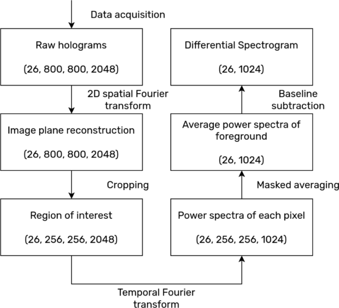
Flowchart of the data processing workflow. The data for each sample undergoes the six data transformation steps outlined. First, 2 d FFT transforms the holograms into reconstructions on the image plane. Next, the data are condensed by cropping around the region of interest (one of the two first-order reconstructions). Next, temporal FFT produces the fluctuation spectra for every pixel. The spectra of the foreground pixels are then averaged. Finally, the log-difference of every spectrum is computed with respect to the averaged baseline spectrum. The numbers in the parentheses in each box indicates the shape of the data, in the order of (number of measurements, pixels in x, pixels in y, number of frames).

The data workflow yields a series of power spectra for each well, as shown in Fig. 4a, and a 2D projection of the same data can be seen in Fig. 4b. In these figures, a snapshot of the dynamics are obtained in the form of a fluctuation spectrum at 1 hour intervals. The changes in the spectra are typically small fractions of the overall spectral weight for a given frequency. Therefore, a log-difference between each spectrum and the log-mean of the baseline spectra was computed. \(S_\text {baseline}\) in Eq. 3 is the log-mean of the four baseline spectra, and \(S’_i\) is the log-difference between each spectrum \(S_i\) and the baseline, \(S_\text {baseline}\).

This log-difference \(\Delta \log (S)\) of the fluctuation power spectra is shown as a differential spectrogram that displays the differential time evolution of the power spectra with respect to the baseline. An example of a spectrogram is shown in Fig. 4c, and an alternative representation showing the log spectral shifts as curves is shown in Fig. 4d. The Doppler shift frequency spectrum has a direct correspondence to the momentum of the scattering body in the sample. Since the Reynolds number in the cytoplasm is very low, viscous force dominates and there is a direct inverse correlation between the size of the scattering body and its velocity (and hence its Doppler shift frequency). As such, different frequency ranges of the Doppler shift spectrum can be mapped to different lengthscales of the scattering body. For instance, the high-frequency bands above 2 Hz correspond to small, fast-moving vesicle and organelle transport, which relate to metabolism; the mid-frequency bands from about 0.05 Hz to 2 Hz correspond to larger organelle movement, e.g. of the nucleus; and the low-frequency ranges below 0.05 Hz correspond to the motions of the cell membrane, such as endocytosis and cell shape change¹⁷. Any external stimuli that can either increase or decrease the level of activity at each lengthscale, in turn, tend to elicit a corresponding change in the spectral weight of the relevant frequency range.

Visualization of the data processing workflow. (a) A 3D visualization of the change in fluctuation spectra of a DLD microcluster infected with 1 kcfu/mL S. enterica over 26 measurements spanning 26 hours. The z-axis indicates the time of data acquisition. The first four power spectra from t = 0 h to t = 4 h hours along the z-axis are the baseline before a treatment (PBS or infection) is applied. The 22 spectra after 0 hours are measured after infection. (b) All 26 power spectra plotted on 2D log-log axes. The time progresses from blue (\(t=0\) h) to red (\(t=26\) h). The direction of spectral shift is indicated by the black arrows. (c) A differential spectrogram. The horizontal and the vertical axes correspond to the x and the z axes of (a). Black line at \(t=0\) h indicates the time of infection. The color scale is the log-difference of the spectral weight, \(\Delta \log (S)\), where red indicates relative increase in the spectral weight, and blue indicates relative decrease. Each line of the contour overlay indicates 0.2 increment in \(\Delta \log (S)\). (d) A plot showing the same information as shown in panel (c). The time progresses from blue (\(t=0\) h) to red (\(t=26\) h), and the black arrows indicate the direction of spectral shift over time.