Dataset
All data utilized in this study were obtained from publicly available open-source online datasets, with no involvement of direct human participation or clinical trials. The COVID-X-ray images were categorized into six classes: Normal (470 images for training and 60 for testing), MERS (135 images for training and 49 for testing), SARS (106 images for training and 27 for testing), Omicron and Delta Variants (111 images for training and 50 for testing), Wild-type SARS-CoV-2 (205 images for training and 52 for testing), and Other Viral Pneumonias (240 images for training and 60 for testing).
The COVID-CT images are categorized into four groups: Normal (954 images for training and 285 for testing), Omicron and Delta Variants (538 images for training and 191 for testing), Wild-type SARS-CoV-2 (450 images for training and 120 for testing), and Other Viral Pneumonias (447 images for training and 118 for testing). These datasets cover various types of viral pneumonia, which are representative of COVID-19 imaging research and aim to simulate the heterogeneity found in real-world multi-center data, despite the limited number of samples in certain categories. They effectively reflect the challenges associated with integrating data across multiple clinical sites.
Method
MLP-Mixer
MLP-Mixer, or Multilayer Perceptron Mixer, is a novel network architecture based on a fully connected layer (MLP), which does not use a convolutional layer or an attention mechanism but instead processes the image through the MLP31. The core of the MLP-Mixer consists of two types of MLPs: Channel-mixing MLPs are responsible for mixing information from different channels at each location.
Token-mixing MLPs: responsible for mixing information between different locations (tokens), as shown in Fig. 1. For each token, token-mixing is performed first to mix spatial information by fusing neighboring pixels within each token. Then, channel-mixing is performed for each dimension to achieve single-position cross-channel feature fusion. When Mixer combines token-mixing and channel-mixing, it accomplishes the transition from token level to channel level by simply transposing the matrix. The alternation of these two mixing types facilitates the exchange and fusion of information across two dimensions. Additionally, Mixer employs skip-connections to add inputs and outputs and uses Layer Normalization (Layer Norm) before the fully connected layer for pre-normalization. A single MLP consists of two fully connected layers with a GELU activation function in between32. The entire computation can be represented as:
$$\begin{aligned} \:Z_{{ * \:,i}} & = X_{{ * \:,i}} + W_{2} \times \:\sigma \:(W_{1} \times \:LN(X)_{{ * \:,i}} ),fori = 1…CY_{{ * \:,i}} \\ & = Z_{{ * \:,i}} + W_{2} \times \:\sigma \:(W_{1} \times \:LN\left( {Z)_{{ * \:,i}} } \right),fori = 1…T \\ \end{aligned}$$
(1)
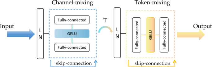
Structure of the MLP-mixer.
In our experiments, we use mixer_b16_224_in21k, where b16 stands for the size of each image block in the model to be 16 × 16 pixels, 224 stands for the size of the input image to be 224 × 224 pixels, and in21k stands for the model to be pre-trained on the ImageNet-21k dataset.
Federal learning
Federated learning is a unique machine learning framework enabling multiple participants to train a shared model collaboratively without centralizing their data in one location33. This type of learning is crucial for protecting user privacy and data security, as it allows data to remain local, and only necessary model updates are shared to the server for aggregation.
FedAvg: FedAvg (Federated Averaging) aggregates model parameters through weighted averaging34. The fundamental concept of FedAvg involves uploading the parameters of local models to a server, where the server calculates the average of all the model parameters and then broadcasts this averaged model back to all local devices.as shown in Fig. 2.
The steps follow: the central server initializes a shared model and distributes its parameters to all k participating clients. Each client then independently trains the received model using its data. After training, each client uploads its model parameters (w) back to the central server. After the central server receives updates from all clients, it computes the average of these updates. This step is the key to FedAvg and is calculated as follows:
$$\:{w}_{t+1}=\frac{1}{N}{\sum\:}_{k=1}^{K}{n}_{k}{w}_{t+1}^{k}$$
(2)
N is the total amount of client data; each client k owns its dataset \(\:{D}_{k}\) which is of size \(\:{n}_{k}\). The global model is updated using these averaged parameters and then sent back to the clients for the next round of training. These steps are repeated until the model achieves the desired accuracy or other stopping conditions are met.
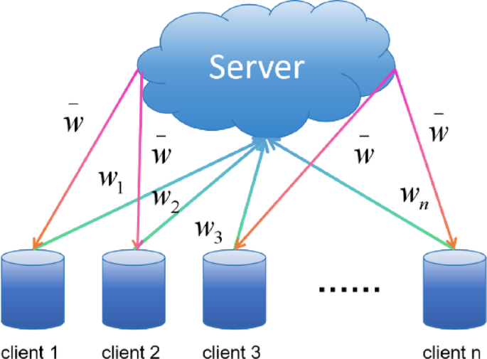
Schematic diagram of the federated averaging (FedAvg) parameter aggregation and distribution process.
Continual learning
Continual learning starts with an initial non-incremental stage \(\:{S}_{0}\) whose model \(\:{M}_{0}\) is trained from the dataset \(\:{D}_{0}=\{{X}_{i},{Y}_{i};i=\text{1,2},\cdots\:,{P}_{0}\}\). \(\:{X}_{i}\) and \(\:{Y}_{i}\) denote the set of samples and the set of labels of the ith data class, respectively, and \(\:{P}_{0}\) denotes the number of classes trained in the stage \(\:{S}_{0}\). For a continual learning process with t stages, it consists of an initial stage and t-1 incremental stages. The incremental phase \(\:{S}_{t}\) uses the model \(\:{M}_{t-1}\) to train the dataset \(\:{D}_{t}=\{{X}_{i},{Y}_{i};i={N}_{t-1}+1,\cdots\:,{N}_{t-1}+{P}_{t}\}\) such that the model can recognize the \(\:{N}_{t}={P}_{0}+{P}_{1}+\cdots\:+{P}_{t}\) categories data35.
Finetune: Finetune, is usually based on a pre-trained model. This process involves adjusting a model’s parameters by continuing training, typically on a new dataset, to enhance the model’s performance on a specific task. In continual learning, the primary application of this approach is to enable the model to learn new tasks while preserving previously acquired knowledge36. Each client simply learns the tasks in sequence.
In the basic finetune process, you have a neural network model pre-trained on some tasks (or multiple tasks), and its parameters are written as θ. Suppose there is a new task, and you wish to continue training this model for this new task while retaining as much as possible of the previously learned knowledge. Given the training data \(\:({x}_{i},{y}_{i})\)for the new task, we define a loss function \(\:L\left(\theta\:\right)\), typically reflecting the performance metric on the new task. The goal of model fine-tuning is to adjust the parameters θ to new values that minimize the loss function:
$$\:{\theta\:}^{\ast\:}={arg}{{min}}_{\theta\:}L\left(\theta\:\right)$$
(3)
In federated learning, applying fine-tuning allows the model to perform incremental learning for each new task by gradually introducing new classes without forgetting old ones. During each local training round, the model fine-tunes the new tasks using cross-entropy loss and utilizes knowledge distillation (not-tue distillation) to retain knowledge from previous tasks. After each communication round, local updates are aggregated to update the global model. Task performance is continuously tracked to ensure that learning new tasks does not negatively affect the performance on old tasks.
LwF: Learning without Forgetting uses only new task data to train the network while maintaining its original functionality37. Relying solely on new task data not only preserves the performance of previous tasks but also acts as a regularization method to enhance the performance of the new task.
We categorize the parameters of the neural network into 3 types: the shared parameter \(\:{\theta\:}_{s}\); the parameter \(\:{\theta\:}_{o}\)on the old task; the specific parameter on the new task and the parameter \(\:{\theta\:}_{n}\) that learns to work well in both the new and the old tasks using only the images and labels of the new task. When training, we first freeze \(\:{\theta\:}_{s}\) and \(\:{\theta\:}_{o}\) and train \(\:{\theta\:}_{n}\) until convergence. Then, train all weights \(\:{\theta\:}_{s}\),\(\:{\theta\:}_{o}\) and \(\:{\theta\:}_{n}\) jointly until convergence.
LwF incorporates two objective functions during training: a loss function for the new task and a loss function to maintain the old knowledge. The hybrid loss function can be expressed as:
$$\:loss={\lambda\:}_{o}{L}_{old}({Y}_{o}\hat,{{Y}_{o}})+{L}_{new}({Y}_{n}\hat,{{Y}_{n}})+R\hat ({{\theta\:}_{s}}\hat,{{\theta\:}_{o}}\hat,{{\theta\:}_{n}})$$
(4)
Losses for new tasks typically use the cross-entropy function, while knowledge distillation losses were used for old tasks.\(\:\lambda\:\)represents the loss of balance weight between the old and new tasks. Adjusting the performance of the old and new tasks can be modified. R is a regular term.
In federated learning, LwF applies incremental learning for each new task, fine-tuning the model to prevent catastrophic forgetting. After each task, the current model is frozen as the old network to retain knowledge from previous tasks. New tasks are trained locally using cross-entropy loss, while knowledge distillation is applied to integrate the knowledge from the old tasks. After each communication round, the local models are aggregated to update the global model.
EWC: Elastic Weight Consolidation is based on Bayesian online learning, which allows the network to retain knowledge about old tasks while learning new ones through elastic consolidation of weights38. When moving from task A to task B, the network aims to minimize the new loss function while imposing specific constraints on the parameters learned from the old task. This is accomplished using the following loss function:
$$\:L\left(\theta\:\right)={L}_{B}\left(\theta\:\right)+{\sum\:}_{i}\frac{\lambda\:}{2}{F}_{i}({\theta\:}_{i}-{\theta\:}_{A,i}^{\ast\:}{)}^{2}$$
(5)
\(\:{L}_{B}\left(\theta\:\right)\) is the loss function for the new task B. \(\:{\theta\:}_{i}\) is the current value of the parameter, while \(\:{\theta\:}_{A,i}^{\ast\:}\) is the value of the parameter obtained after task A. \(\:{F}_{i}\) is the Fisher information about the parameter \(\:{\theta\:}_{i}\), which measures the importance of the parameter \(\:{\theta\:}_{i}\) in task A. \(\:\lambda\:\) is a hyperparameter that controls the influence of the old task on learning the new task. The Fisher information matrix F is the expected value of the variance of the loss function L concerning the gradient of the parameter θ:
$$\:{F}_{i}=E\left[(\frac{\partial\:{L}_{A}}{\partial\:{\theta\:}_{i}}{)}^{2}\right]$$
(6)
Suppose a parameter is critical in the old task. In that case, the value of the Fisher information for this parameter will be large, and the EWC method will reduce the variation of these parameters by increasing the corresponding regularization term in the loss function.
When applying the EWC to federated learning, the model learns new tasks through incremental training while protecting the knowledge of old tasks via EWC loss. After each task, the model’s parameter mean and Fisher information matrix are saved, and a penalty term is computed to prevent excessive changes to important parameters. Through local training and EWC regularization, the learning of new tasks is balanced with the retention of knowledge from old tasks. Additionally, after each communication round, the locally updated model weights are aggregated, ensuring the global model can effectively adapt to all tasks and avoid catastrophic forgetting.
BEEF: Bi-compatible class-incremental Learning via Energy-Based Expansion and Fusion combines the expansion and optimization of energy functions and the integration of old and new knowledge to solve the problem of “catastrophic forgetting” in incremental learning39. BEEF introduces the energy function \(\:E(x;{\theta\:}_{y})\), which measures the degree of match between a sample and its corresponding category. When the model encounters a new class, by minimizing the energy value of the sample under the correct class, the model can dynamically expand and adapt to the new class. At the same time, to prevent forgetting the old class when introducing a new class and keep the energy levels of the old and new classes balanced, BEEF designs an objective function:
$$\:{{min}}_{\theta\:}{\sum\:}_{i=1}^{N}{E}_{({x}_{i},{y}_{i})}\left[E\right({x}_{i};{\theta\:}_{{y}_{i}}\left)\right]+\lambda\:{\sum\:}_{j=1}^{K}{E}_{{x}_{j}\sim{p}_{j}}[E({x}_{j};{\theta\:}_{{y}_{j}})]$$
(7)
In addition, BEEF ensures that introducing new classes does not negatively affect the old classes through a dual compatibility mechanism, maintaining the overall stability of the model. To better integrate the old and new knowledge, BEEF employs a fusion mechanism that combines the energy functions of the old and new classes, thus realizing a smooth transition between the old and new knowledge.
$$\:\stackrel{\sim}{E}(x;\theta\:)=\alpha\:{E}_{old}(x;{\theta\:}_{old})+(1-\alpha\:){E}_{new}(x;{\theta\:}_{new})$$
(8)
In federated learning, BEEF applies incremental learning by fine-tuning the model for each new task while preserving knowledge from previous tasks. During local training, the model uses cross-entropy loss for new tasks and an energy-based regularization loss to prevent excessive parameter updates that could disrupt previously learned tasks. The energy is calculated by analyzing the magnitude of parameter updates, and a fusion approach is used to blend the old and new energy values, ensuring a balance between new learning and knowledge retention. After each communication round, local updates from clients are aggregated to update the global model.
Evaluation indicators
Task accuracy is very important in continual learning tasks based on federated learning. We use the same average accuracy metric as previous studies to evaluate the model’s performance40. We define it as the model’s accuracy on the kth task test set after learning i tasks sequentially.
The average accuracy \(\:{A}_{i}\) measures the performance of the continual learning algorithm across all test sets after learning i tasks and can be expressed as follows:
$$\:{A}_{i}=\frac{1}{i}{\sum\:}_{k=1}^{i}{a}_{i,k}$$
(9)
When the amount of test data for each class differs, a weighted version of Eq. (9) is required.
Additionally, to study the issue of catastrophic forgetting in continual learning, we introduce the forgetting measure F41. F is an important metric for quantifying the extent to which a model forgets old task knowledge after learning new tasks. To comprehensively evaluate the model’s ability to retain knowledge, we define the forgetting measure F as the average forgetting across all previous tasks after learning the k-th task.
The forgetting measure Fk is computed using the following formula:
$$\:{F}_{k}=\frac{1}{k-1}{\sum\:}_{j=1}^{k-1}{f}_{k}^{j}$$
(10)
where \(\:{F}_{k}\) represents the average forgetting of the previous \(\:k-1\) tasks after learning the k-th task, and \(\:{f}_{k}^{j}\) quantifies the forgetting of the j-th task after learning the k-th task.
Next, to compute the forgetting for each task, we use the following formula:
$$\:{f}_{k}^{j}=\frac{1}{\left|{C}_{j}\right|}\sum\:_{c\in\:{C}_{j}}\underset{t\in\:\left\{1,\cdots\:,N-1\right\}}{\text{max}}\left({A}_{c}^{\left(n\right)}-{A}_{c}^{\left(N\right)}\right)$$
(11)
where \(\:{C}_{j}\) is the set of classes related to the j-th task, \(\:{A}_{c}^{\left(n\right)}\) is the accuracy on class c during the n-th learning phase, and \(\:{A}_{c}^{\left(N\right)}\) is the final accuracy on class c after all tasks have been learned. By comparing the accuracy differences across learning phases, we can quantify the forgetting of the j-th task.
Experiment
In this experiment, we established a novel Federated Continual Learning framework for infectious disease prediction and simulated a Transnational Infectious Disease Prediction Model based on this framework as shown in Fig. 3. This model realizes a multi-client-participatory federated learning system with a focus on data privacy. The system simulates 3 and 6 internatioanal clients, all connected to a central server. These clients may represent different healthcare institutions or data centers, which collaboratively participate in building an infectious disease prediction model through federated learning.
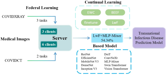
Framework and procedure of federated continual learning for transnational infectious disease prediction.
On the server side, various machine learning strategies are employed to optimize the performance of the model. Continual learning strategies such as EWC, LwF, BEEF and Finetune are integrated to enhance the model’s adaptability and efficiency. By incorporating these techniques, the model is capable of processing data from diverse clients while ensuring data privacy and guaranteeing the accuracy42. Multiple models have been utilized within the system for performance evaluation. They are 10 pre-trained models transferred and fine-tuned from the timm library, allowing for comprehensive analysis and optimization of the predictive capabilities:
Swin Transformer: Swin Transformer is a Transformer-based visual model that uses a localized attention mechanism called “windowing,” making it more efficient in processing large images43. In our experiments, we use the model swin_small_patch4_window7_224.
ResNet: ResNet is a Convolutional Neural Network (CNN) architecture that is part of the Residual Network (ResNet) family. It achieves this by introducing so-called “residual chunks”, which effectively allow the network to learn a constant mapping, which helps to transfer information between layers and avoids the problem of vanishing gradients problem44. In our experiments, we use the model resnet18.
EfficientNet: EfficientNet is an efficient convolutional neural network architecture designed based on an idea known as the “composite scaling method”, which systematically investigates the scaling of the network’s width, depth, and resolution to find an equilibrium that allows the model to achieve optimal performance under different computational budgets45. In our experiments, we use the model efficientnet_b0.
MobileNet V3: MobileNetV3 is an efficient convolutional neural network architecture optimized for mobile and edge devices that automatically finds the optimal structure for a given hardware through Network Architecture Search (NAS)46. In our experiments, we use the model mobilenetv3_large_100.
Vision Transformer: Vision Transformer (ViT) is an innovative image processing model that applies the self-attention mechanism (with Transformer as the core component) to the field of computer vision47. In our experiments, we use the model vit_base_patch16_224.
ConvNeXt: ConvNeXt is based on design insights from the Transformer architecture and improves the performance and efficiency of the model by redesigning and optimizing key components in standard convolutional networks48. In our experiments, we use the model convnext_base.
DenseNet: DenseNet is a convolutional neural network architecture characterized by dense connections between each layer. This design significantly enhances gradient propagation, reduces the number of parameters, and increases the network’s efficiency and effectiveness49. In our experiments, we use the model densenet121.
Inception V3: Inception V3 is an advanced convolutional neural network architecture that can capture different scale features of an image within the same layer by introducing multi-scale processing techniques and convolutional decomposition to improve feature representation50. In our experiments, we use the model inception_v3.
DeiT: DeiT (Data-efficient Image Transformers) is a Transformer model designed for image categorization that improves data efficiency using knowledge distillation techniques, allowing the model to learn effective visual representations even with less data51. In our experiments, we use the model deit_small_patch16_224.
There is also the MLP-Mixer model, which we described earlier. In our experiments, we use the model mixer_b16_224_in21k.
Our experiments were conducted on two 4090 GPUs, where we set 3 incremental learning tasks for COVIDXRAY(6 classes) and 2 for COVIDCT(4 classes). We configured the experiment for federated learning with both 3 and 6 clients. Each client was set to undergo 32 local training epochs, with 15 communication rounds. As for the dataset, we performed data transformations on the pre-split training and test sets, including resizing and normalization, and conducted label mapping.
In our experiment, data partitioning was done using a Non-IID (Non-Independent and Identically Distributed) approach, specifically using the Dirichlet distribution to allocate the data52. By setting beta to 0.5, the data is not evenly distributed across clients; instead, there are variations in the data distribution between clients. Each client’s dataset contains samples from multiple classes, but the number of samples per class varies. The task partitioning and incremental learning process is carried out by progressively introducing new classes. We first determine the number of classes for the initial task, and these classes are trained in the model first. Subsequently, each task introduces more classes, allowing the model to gradually encounter more classes and adapt to them. The training for each task is done independently, and as the number of classes increases, the dataset for each task expands, ensuring that each task builds on the previous one with new learning objectives.
In the process of local training and global aggregation, each client independently trains its model and updates its weights. These local updates are periodically sent to a central server. Upon receiving the local models from the clients, the server aggregates the weights. The server averages the model weights from all clients, resulting in an updated global model, which is then sent back to the clients. The clients receive the global model and continue with the next round of local training. This process is repeated, with each round involving local training and global aggregation to gradually improve the model’s performance.


