Revisiting the link between COVID-19 incidence and infection fatality rate during the first pandemic wave

Categories: Disease & Virus

May 5, 2025

SAPRIS-SERO study

This study used the data of the SAPRIS-SERO serosurvey, previously described^18,20. SAPRIS-SERO was built on SAPRIS (“SAnté, Perception, pratiques, Relations et Inégalités Sociales en population générale pendant la crise COVID-19”), a cohort whose inclusions began in March 2020, which studied epidemiological and sociological aspects of the COVID-19 epidemic in France²¹. The adult participants of SAPRIS were recruited from three cohorts based on the general population (without particular selection on a disease):

The cohort NutriNet-Santé focused on nutrition, with online follow-up. It included 170,000 participants at the start of the study in 2009²².
The cohort CONSTANCES was set up in 2012 and included 204,973 adults, selected to be a representative sample of the French adult population²³.
E3N/E4N is a multi-generational adult cohort including 113,000 persons: the women recruited at the start of the study (1990), their children, and the fathers of these children²⁴.

All participants from the initial cohorts who had regular internet access and were still being followed in 2020 were invited to participate in the SAPRIS study, which involved self-administered questionnaires during the first wave²¹. These questionnaires covered demographic information and the history of SARS-CoV-2 testing by RT-PCR. A total of 93,610 SAPRIS participants were over 20, completed the questionnaires, and resided in metropolitan France. These participants were then invited to join the SAPRIS-SERO study by collecting a single dried-blood spot sample themselves. The samples were sent to a virology laboratory (Unité des virus émergents, Marseille, France) for serological analysis using the commercial ELISA test (Euroimmun, Lübeck, Germany), which detects anti-SARS-CoV-2 IgG antibodies targeting the S1 domain of the spike protein. The ELISA assays performed on dried-blood spot samples demonstrated a sensitivity of 98.1 to 100% and a specificity of 99.3 to 100% when compared to conventional serum assays as a standard^25,26.

External data

The results of two independent French seroprevalence studies were used as prior distributions for national seroprevalence (metropolitan France)^17,27. The results of a diagnostic study concerning the ELISA test (IgG anti-S1 from Euroimmun) were used as prior distributions for sensitivity and specificity²⁸.

The French population structure by age and by administrative department came from the census of January first, 2020 (Insee, Institut national de la statistique et des études économiques)²⁹. The data about COVID-19-related hospitalizations during the first semester (before July first, 2020) by administrative department were obtained from the SI-VIC database, the exhaustive national inpatient surveillance system used during the pandemic³⁰. The data about general population mortality (including deaths occurring in nursing homes) attributed to COVID-19 during the first semester (before July first, 2020) were obtained from the CépiDc (Centre d’épidémiologie sur les causes médicales de décès), online (open data) or directly³¹. Raw diabetes prevalence in French departments in 2019 (pre-pandemic) was provided by Santé Publique France (open data), based on an exhaustive monitoring of anti-diabetic drugs use (Système national des données de santé)³². The number of ICU (intensive care unit) beds per inhabitant in 2019 (pre-pandemic) was obtained from the DREES (Direction de la recherche, des études, de l’évaluation et des statistiques)³³.

Identification of causal effects

The relation between incidence and IFR is confounded, as the determinants of IFR may share socio-economic causes with incidence at the scale of departments. Typically, wealthier departments could have a population which travels more (possibly increasing incidence) and which is healthier (decreasing IFR), participating in a spurious negative association between incidence and IFR. Thus, IFR was adjusted (by conditioning and averaging, as described in the Statistical model section) for the main determinants of COVID-19 outcome: prevalence of diabetes (as a surrogate for obesity), proportion of the population over 60, and number of intensive care beds per inhabitant^8,9,34,35. Prevalence of diabetes was chosen as a surrogate for obesity because it is easier to quantify precisely (through data on the sale of diabetes medication).

Figure 1 features a causal graph representing departmental incidence (X), IFR or IHR (Y), unobserved socio-economic variables (C), and the determinants of COVID-19 outcome (according to^8,9,34,35). Our most critical assumptions, which are included in the graph, are:

Age and diabetes are the main individual risk factors for COVID-19 severity, influencing hospitalization and mortality.
The determinants of IFR and IHR at the departmental scale act through the prevalence of these individual risk factors, through incidence, or through the number of intensive care beds per inhabitant (the latter having a potentially decisive role for IFR but acting as a surrogate for hospital beds when considering IHR).

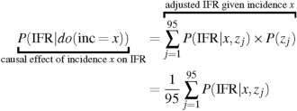
Given this causal graph (Fig. 1), the set {Diab., Age, Beds} satisfies the back-door criterion relative to (X, Y) and allows for estimating the causal effect of X on Y despite the presence of unobserved socio-economic variables, using the back-door adjustment formula (Eq. 1)³⁶. Let $P(\text {IFR}|do(\text {inc}=x))$ denote this causal effect, which is the distribution of departmental IFRs if incidence (inc) was artificially set to the value x for all the departments, without any other modification. With $z_j$ denoting the vector of covariates for a department j, and because the distribution of these covariates in the 95 departments of metropolitan France is known ($P(z_j) = \frac{1}{95}$ for all j),

(1)

The target of this study was the average causal effect of an incidence shift from 3 to 9%:

$$\begin{aligned} E[\text {IFR}|do(\text {inc}=9\%)] – E[\text {IFR}|do(\text {inc}=3\%)] \end{aligned}$$

(2)

This average causal effect corresponds to the expected difference in IFR when artificially setting incidence to 9% versus 3% in a department of metropolitan France (without changing anything else than incidence). The same formula was used to identify the average causal effect of this incidence shift on IHR.

Statistical model

We used a Bayesian statistical framework to leverage multiple sources of data and to account for uncertainty surrounding the latent variables when used in regressions (such as incidence and IFR). An overview of the model is featured in Fig. 2, where the equations of the model are referenced next to the variables.

In the remainder of this section, prior distributions are not always explicitly written. If so, the latter are uniform. Age groups are indexed by the letter i ($i = 0$ for individuals aged 20 to 59, and $i = 1$ for individuals aged over 60). The departments are indexed by the letter j, ranging from 1 to 95.

For an age group i and a department j, the participants without a positive RT-PCR nor missing data on department contributed to the estimation of seroprevalence $s_{i,j}$, considering $N_{i,j}$ the number of these participants, and $y_{i,j}$ the number of positive serological tests:

$$\begin{aligned} y_{i,j} \sim \text {B}(N_{i,j}, s_{i,j}) \end{aligned}$$

(3)

Seroprevalence at the scale of metropolitan France ($\text {sero}_{\text {France}}$) was obtained by post-stratification from $s_{i,j}$ and $\text {pop}_{i,j}$, the size of the population corresponding to this group:

$$\begin{aligned} \text {sero}_{\text {France}} = \frac{\sum _{i,j} \text {pop}_{i,j} \times s_{i,j}}{\sum _{i,j} \text {pop}_{i,j}} \end{aligned}$$

(4)

Seroprevalence estimates from other surveys were incorporated using beta distributions:

$$\begin{aligned} \begin{aligned} \text {sero}_{\text {France}}&\sim \text {Beta}(101, 1948) & \text {(implies a 95}\%\text { CI of 4.02–5.89}\%\text { [17])}\\ \text {sero}_{\text {France}}&\sim \text {Beta}(1147, 17212) & \text {(implies a 95}\%\text { CI of 5.90–6.60}\% \text {[27])} \end{aligned} \end{aligned}$$

(5)

For an age group i and a department j, incidence (cumulated over the first semester) was denoted $p_{i,j}$. Seroprevalence $s_{i,j}$ was linked to incidence $p_{i,j}$ and to the sensitivity (Se) and specificity (Sp) of the serological test:

$$\begin{aligned} s_{i,j} = Se \times p_{i,j} + (1 – Sp) \times (1 – p_{i,j}) \end{aligned}$$

(6)

Prior distributions for sensitivity and specificity originated from²⁸:

$$\begin{aligned} \begin{aligned}&\text {Se} \sim \text {Beta}(585, 56) & \text {(implies a 95}\% \text {CI of 89.0–93.3}\%)\\&\text {Sp} \sim \text {Beta}(953, 15) & \text {(implies a 95}\% \text {CI of 97.6–99.1}\%) \end{aligned} \end{aligned}$$

(7)

The participants with a positive RT-PCR contributed to the likelihood of sensitivity. With $N_{\text {se}}$ and $y_{\text {se}}$ the number of total and positive (respectively) serological tests in this group,

$$\begin{aligned} y_{\text {se}}&\sim \text {B}(N_{\text {se}}, \text {Se}) \end{aligned}$$

(8)

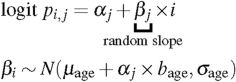
Incidence $p_{i,j}$ was modeled on the logit scale. As it was suggested that older persons could be under-represented in the population of infected persons at the early stages of the epidemic¹⁹, every department had a unique log-odds ratio for age over 60 ($\beta _j$), possibly influenced by its intercept $\alpha _j$ (logit of incidence in the 20-59 in the department j) through a linear regression with intercept $\mu _{\text {age}}$, slope $b_{\text {age}}$ and standard deviation $\sigma _{\text {age}}$ (hierarchical modeling, $\beta _j$ is a random effect):

(9)

The $\alpha _j$ departmental intercepts entailed spatial auto-correlation through an ICAR (intrinsic conditional auto-regressive) component $\phi _j$(as described and implemented in this reference³⁷), associated with an overall intercept $\mu _{\alpha }$ and a scale parameter $\sigma _{\phi }$ representing the amount of spatial correlation:

$$\begin{aligned} \begin{aligned}&\alpha _j = \mu _{\alpha } + \phi _j \times \sigma _{\phi }\\&\sigma _{\phi } \sim \text {Exponential}(1) & \text {(weakly informative prior on }\sigma _{\phi }) \end{aligned} \end{aligned}$$

(10)

The proportion $\text {age}_{\text {infected,j}}$ of persons over 60 among those infected in a department j was reconstructed from $p_{i,j}$ and from $\text {age}_{\text {pop},j} = \frac{\text {pop}_{1,j}}{\text {pop}_{1,j} + \text {pop}_{0,j}}$ (the proportion of persons above 60 in the population of the department j):

$$\begin{aligned} \text {age}_{\text {infected,j}} = \frac{p_{1,j} \times \text {age}_{\text {pop},j}}{p_{1,j} \times \text {age}_{\text {pop},j} + p_{0,j} \times (1 – \text {age}_{\text {pop},j})} \end{aligned}$$

(11)

For a given incidence in the persons under 60, we estimated an expected proportion of persons over 60 among those infected for a department with the same age structure as metropolitan France. This expected proportion was reconstructed from the coefficients $\mu _{age}$, $\beta _{age}$, and $\sigma _{age}$ (Eq. 9), according to a procedure described in Supplementary Information 1 (“Computation of expectations”). This analysis aimed to illustrate the dependence between incidence in people under 60 and incidence in those over 60, and its possible consequences for IFR.

The K participants with a positive RT-PCR and no missing data concerning the department contributed directly to incidence. With $\text {IS}_k$ being the infection status of the participant k ($\text {IS}_k$ is always equal to 1 in this positive RT-PCR group),

$${\text{IS}}_{k} \sim {\text{Bern}}(p_{{i,j}} )\;;{\text{(For }}k = 1, \ldots ,K)$$

(12)

Departmental incidence $\text {inc}_j$ was obtained by post-stratification from $p_{i,j}$ and $\text {pop}_{i,j}$:

$$\begin{aligned} \text {inc}_j = \frac{\sum _{i} \text {pop}_{i,j} \times p_{i, j}}{\sum _{i} \text {pop}_{j}} \end{aligned}$$

(13)

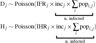
For a department j, the counts of deaths ($\text {D}_j$) and hospitalizations ($\text {H}_j$) of the first semester were modeled with Poisson regressions:

(14)

Departmental IFRs and IHRs were modeled as logistic functions of linear predictors $g_\text {IFR}(j)$ and $g_\text {IHR}(j)$, ranging respectively from 0 to 5% and from 0 to 10%:

$$\begin{aligned} \begin{aligned} \text {IFR}_j&= \frac{0.05}{1 + e^{- g_\text {IFR}(j)}} & \text {(logistic function ranging from 0}\,\text { to 5}\%)\\ \text {IHR}_j&= \frac{0.10}{1 + e^{- g_\text {IHR}(j)}} & \text {(logistic function ranging from 0}\,\text { to 10}\%) \end{aligned} \end{aligned}$$

(15)

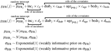
These linear predictors included a departmental random intercept, a slope representing the role of incidence, and coefficients associated with the covariates (prevalence of diabetes, number of intensive care beds per inhabitant and proportion of the population over 60). With $\text {diab}_j$, $\text {age}_{\text {pop},j}$, and $\text {beds}_j$ being the covariates for the department j,

(16)

The coefficients of Eq. (16) were used to compute $E[\text {IFR}|do(\text {inc}=x)]$, and subsequently the average causal effect of incidence on IFR, as described in Supplementary Information 1 (“Reconstruction of expectations” section). The same procedure was used to compute the effect of incidence on IHR.

Algorithm and software

The data management was done using R version 4.3.1, and the modeling was performed with Stan (R package cmdstanr version 0.5.3), which implements Hamiltonian Monte Carlo (HMC)^38,39. The models for the random coefficients ($\beta _j$, $\mu _{\text {IFR}_j}$ and $\mu _{\text {IFR}_j}$) employed non-centered parameterizations to improve HMC convergence⁴⁰. The Monte Carlo sampling consisted of 8 chains of 2,000 iterations each (including 1,000 warm up iterations). Trace plots, ${\hat{R}}$ statistics and effective Monte Carlo sample sizes provided by Stan were used to assess convergence. Posterior predictive checks are provided in Supplementary Information 2. The model’s code (in Stan) is provided in Supplementary Code 1 and in a GitHub repository (https://github.com/bglemain/does-hospital-overload).

Ethical approval and consent to participate

Ethical approval and written or electronic informed consent were obtained from each participant before enrollment in the original cohort. The SAPRIS-SERO study was approved by the Sud-Mediterranée III ethics committee (approval 20.04.22.74247) and electronic informed consent was obtained from all participants for dried blood spot testing. The study was registered (#NCT04392388). All methods were performed in accordance with the relevant guidelines and regulations.

Source link