Modified variations of HFEA with ITT and Futures / Lifecycle Investing with Fashionable Portfolio Principle - Web page 65

skierincolorado wrote: ↑Wed Sep 11, 2024 9:45 am

comeinvest wrote: ↑Wed Sep 11, 2024 1:40 am

skierincolorado wrote: ↑Tue Sep 10, 2024 4:15 pm

comeinvest wrote: ↑Tue Sep 10, 2024 3:30 pm

skierincolorado wrote: ↑Tue Sep 10, 2024 10:30 am
I feel you are in all probability underestimating the normality of returns. Time heals as a result of the anticipated return is constructive, not high-autocorrelation. The fallacy of time diversification confirmed by Samuelson is broadly accepted in educational finance, so I might be very cautious and cautious about disregarding it. Though the idea of normality is little doubt flawed, it could be an in depth sufficient approximation to show the fallacy of time diversification.

I feel it is each a imply reverting part, overreactions that for instance manifest themselves whenever you take a look at dividends or smoothed earnings that fluctuate a lot lower than share costs; and the truth that the anticipated return is constructive annually. Which one would not matter. If after 30-40 years all of your outcomes or a 99% percentile of your probabilistic ultimate wealth distribution are above that of an alternate asset allocation, then you do not care. If with technique B you’ll have someplace between say 2x and 10x the cash in comparison with technique A, then you do not care in regards to the excessive dispersion between 2x and 10x. Time diversification is the entire premise of this thread. The “fallacy” of time diversification is accepted in “educational” finance that’s primarily based on assumptions indifferent from actuality; and I feel the authors of the papers that display one thing alongside these strains know that it is only a arithmetic train that does not replicate actuality. Maybe it has some applicability for up to some years value of serial returns, however not for longer intervals. Like I stated, I feel a greater means of assessing tail danger is to assume by means of actual macroeconomic and finance situations primarily based on life like assumptions.

The authors absolutely settle for that point diversification is a fallacy. And they’re clear that their utilization of the phrase refers to one thing solely completely different. You do care if leverage will increase the dispersion of your ultimate wealth from 4-10x of present wealth to 2-30x of present wealth. The potential lack of utility from 4x to 2x could also be greater than the potential achieve in utility from 10x to 30x, relying on RRA. Whereas for a extremely wealth particular person, there could also be little lack of utility from 4x to 2x present wealth, there would even be little achieve in utility from 10x to 30x. If in case you have no utility from any change in wealth in anyway, there is not any profit to take a position in any respect.

I feel you may discover Samuelson’s proof of the fallacy of time diversifcation is convincing should you look into it some extra. The Lifecycle Investing ebook’s concentrate on human capital can be fairly convincing as the first justification for leverage. I do not assume relative danger aversions under 1 make a lot sense rationally. As such, I do not assume leveraging equities with restricted/no future earngings makes a lot sense. Being leveraged general, like 100% equities 150% ITT, might nonetheless make sense. In actual fact, the upper sharpe might justify as excessive because the 140/250 you’ve got, however I might guess extra like 100/150 or 120/200.

I perceive that the principle level of the ebook and the definition of “time diversification” applies to the buildup section. As we found, the utility perform could also be exhausting to outline, and every particular person situation is completely different. Whether or not the optimum asset allocation with no cash addition from exterior is 100% or 135% equities and the way a lot ITT so as to add and whether or not that justifies increased or decrease allocation to equities, relies upon closely on assumptions as we found on this thread. However once I see a system that’s primarily based on uncorrelated return sequences, I simply skip the article and the outcomes. For me it is a waste of time. Any mathematical mannequin that’s alleged to replicate the actual world must be primarily based on actual information. It is in all probability finest to straight backtest with historic information, after all not blindly however with sensical changes the place wanted, moderately than create a simplified mannequin and blindly plug numbers into it.

skierincolorado wrote: ↑Tue Sep 10, 2024 4:15 pm
I’m fairly skeptical that any autocorrelation of returns would considerably have an effect on the conclusion over the timeframe we’re speaking about (30-40 years for most individuals, much less if we embody withdrawals).

I do not know the way massive the distinction can be. I might at all times go by actual historic information, if there have been a distinction. I suppose one of many variations is likely to be that the simplified mathematical mannequin would permit the situation of three GFC (2007-2009) market crashes, or the 1987 the 2000-2002 and the 2007-2009 drawdowns to happen in sequence over 6 years, as one doable end result. The actual life likelihood of that is exhausting to derive from historical past due to the singular nature of most main occasions in trendy historical past; however should you assume by means of that situation from a macroeconomic and asset valuation perspective, an 80%+ fairness market drawdown is tough to think about except one thing occurs so that you’ve got larger issues than your portfolio. Likewise, the usually distributed mannequin would permit situations with no restoration; historical past has by no means seen an fairness market with no restoration usually inside just a few years, except belongings had been confiscated no matter leverage wherein case you could possibly argue you’ve got an asymmetrical benefit should you use leverage. If you happen to take a look at charts that present valuation vs. 5-year or 10-year efficiency that you’ve got seen, there’s a excessive chance of robust efficiency after a meltdown (which normally comes with low valuations). The ten-year correlation is kind of robust. Your mannequin would not replicate that.

skierincolorado wrote: ↑Tue Sep 10, 2024 4:15 pm
Since that is very a lot in opposition to accepted educational concept – even probably the most danger tolerant theorists – I feel it requires extraordinary proof. I do not assume you possibly can dismiss primarily based on the concept of autocorrelation with out some empirical and theoretical investigation.

I am not conscious of generally “accepted” educational concept or monetary recommendation. There may be arithmetic, there’s analysis, and there’s the historical past of the inventory market, and all are publicly accessible for the investigative minds to attract their conclusions. The historical past of the inventory market result in a trillion completely different fashions and makes an attempt at predicting its future, however nearly nothing would persuade me to belief a mannequin derived from historical past greater than the historic information itself. I do not even need to hassle with ideas like autocorrelation which are strategy to difficult for me in the intervening time.

If you happen to argue that any individual with a 30 yr funding horizon ought to have the identical allocation to equities as somebody with a 2 yr funding horizon, when historical past had quite a few market crashes throughout 2 yr horizons however by no means noticed an actual loss over 30 years even should you poured all of your belongings without delay into the market at one of many market peaks, then I feel that will be fairly an extravagant recommendation. Like I stated that has nothing to do with the idea of “time diversification” referenced earlier.

I imply we will speculate all we would like. Extraordinary claims require extraordinary proof. Let’s take a look at the information.

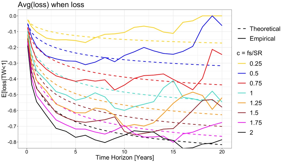
Simulations over rolling 20 yr home windows during the last 95 years present that the terminal returns behave remarkably just like Samuelson’s concept and the theoretical return from 20 random impartial annual returns (regular). There may be little proof of imply reversion in anyway. The legend represents proportion of the kelley criterion. The dashed strains are the likelihood of loss predicted by random impartial annual returns with a stdev of 17% and ER of 8%. The strong strains are the precise likelihood of loss over the rolling home windows for the historic information throughout which stdev was 17% and ER was 8%.

At time horizons so long as 15 years the likelihood of loss is considerably HIGHER than a standard random distribution of annual returns would predict. There was zero imply reversion on a horizon of 15 years during the last 95 years of information. On a horizon of 20 years there’s some slight proof of imply reversion, particularly for decrease leverage at or under 1 kelley crit. Nonetheless, this can be luck because of the small pattern measurement of rolling 20 yr home windows. There are solely 5 absolutely impartial 20 yr home windows, versus 10 10 yr home windows.

Thanks! I feel these a wonderful charts.
Bt Kelly criterion you imply the optimum fraction per Kelly? So “1” in you legend would correspond to the optimum leverage for these 95 years, in all probability someplace between 2 and three? And something above “1” in your legend can be irrelevant in apply?

I am undecided how “imply reversion” would present in your charts, and I did not even outline it in my feedback. I feel imply reversion would refer for instance to valuation ratios, which are clearly vary certain, fluctuating across the financial development and earnings development path. I feel the expansion price can be thought of vary certain or imply reverting; however clearly the GDP or company earnings themself can expertise setbacks or acceleration and should not imply reverting in that sense. However that type of evaluation and decomposition is difficult and never related to the query of shortfall danger, so long as now we have these charts.

We will see that the empirical likelihood of loss is decrease than the mannequin likelihood of loss as much as ca. 5 years. I feel that’s as a result of the actual outcomes present extra sudden drawdowns, however much less steadily than the mannequin predicts primarily based on regular distribution. That truth is effectively is aware of, however likewise in and by itself not likely related, so long as now we have the information and the charts of danger and returns for longer intervals. Over medium lengthy intervals, this asymmetry appears to offset and easy out, because the strong and the dashed strains come nearer and fluctuate round one another.

Again to the unique query of optimum leverage and danger for portfolio with no extra future funding, and if the funding horizon must be an enter to the asset allocation, particularly to the leverage ratio.
I do not know, but when a leverage of for instance 135% can be 0.5x the Kelly optimum, then my likelihood of loss can be zero per the chart for a 20 yr funding horizon. Whether or not the strong blue line is above or under the dashed blue line might be not likely related, as a result of we all know that the actual life likelihood is rarely zero, as a result of something can occur on this planet. However the strains are shut sufficient.
Fortunately your 95 years would come with the height earlier than the 1929 crash, which is sweet as a result of then now we have that situation additionally lined by the charts.

So my takeaway is 1a. likelihood of loss approaches zero the longer the funding horizon, with each mannequin and actual life information, an extended as leverage is under the Kelly optimum; 1b. for no or reasonable leverage, the likelihood of loss goes to close zero or zero at in regards to the 20 yr mark; 2. after about 15 years, the actual life share portfolio losses change into measurably smaller than the mannequin predicted losses. (Leverage to Kelly optimum ratio of “1” appears to be an outlier; however I suppose solely 0.25, 0.5, and 0.75 are related as a result of no person sane of their minds would go along with 1 or past with their very own cash.)

So concerning the actual life vs. mannequin variations, I feel the truth that the actual life likelihood of loss at 20 years is zero could also be both an artifact of restricted historical past, or resulting from incorrect mannequin assumptions. I feel it’s moderately irrelevant which one it’s.
I feel the extra related and extra noticeable distinction is the upswing of the yellow, blue and purple strong strains vs. their dashed counterparts between 15 and 20 years within the second chart. Whether or not that may be attributed to “imply reversion” of underlying financial or monetary parameters in no matter sense, just isn’t related for the implications to the asset allocation.
In actual fact, the dashed strains would in all probability flatted, however hold lowering without end within the second chart; whereas the strong strains clearly do not, and the smaller the leverage ratio the earlier the upswing begins.

For function of asset allocation and portfolio leverage, I am undecided how related the rising magnitude of the tail danger loss per the dashed strains can be, on condition that the likelihood of that loss occurring approaches zero with time. I suppose an argument for elevated tail danger with rising time horizon may very well be made per the mannequin outcomes, scaring away risk-adverse buyers from 100% equities asset allocations, not to mention leverage portfolios. However though something (together with the destruction of the world) can occur after all, that is precisely the manifestation of the shortcomings of the traditional and uncorrelated mannequin distribution assumptions. The actual life information clearly do not present that tail danger, as loss possibilities go to zero, and share losses change into smaller with rising time horizon, and ultimately disappear. Because of this, increased leverage ratios must be chosen for longer time horizons. If you happen to had been to increase the charts to 30 or 35 years, the variations would change into even far more clear.